Erstellen von Zeitreihenprognose für SCM mit R tidymodels

Vorbereitende Arbeiten

Pakete laden

library(sysfonts)
library(showtext)
library(thematic)
library(corrplot)
library(hardhat)
library(tsibble)
library(skimr)
library(tidyverse)
library(tidymodels)

# Konflikte zwischen tidymodels und anderen Paketen lösen
tidymodels_prefer()

# Standardthema für ggplot2-Plots festlegen
ggplot2::theme_set(theme_dv())

Daten laden

daten <- read_csv(file = "data/sales1_ML.csv")

Datenanalyse als Teil der Modellierung

Explorative Datenanalyse (EDA)

head(daten)

# A tibble: 6 × 14
  date       store_name dept  family subfamily section brand size  color product
  <date>     <chr>      <chr> <chr>  <chr>     <chr>   <chr> <chr> <chr> <chr>  
1 2021-01-01 store_1    depa… famil… subfamil… sectio… bran… size… colo… sku_1  
2 2021-01-01 store_1    depa… famil… subfamil… sectio… bran… size… colo… sku_2  
3 2021-01-01 store_1    depa… famil… subfamil… sectio… bran… size… colo… sku_3  
4 2021-01-01 store_1    depa… famil… subfamil… sectio… bran… size… colo… sku_4  
5 2021-01-01 store_1    depa… famil… subfamil… sectio… bran… size… colo… sku_5  
6 2021-01-01 store_1    depa… famil… subfamil… sectio… bran… size… colo… sku_4  
# ℹ 4 more variables: unit_price <dbl>, revenue <dbl>, price_total <dbl>,
#   qty <dbl>

glimpse(daten)

Rows: 530,765
Columns: 14
$ date        <date> 2021-01-01, 2021-01-01, 2021-01-01, 2021-01-01, 2021-01-0…
$ store_name  <chr> "store_1", "store_1", "store_1", "store_1", "store_1", "st…
$ dept        <chr> "department_1", "department_2", "department_1", "departmen…
$ family      <chr> "family_1", "family_2", "family_3", "family_4", "family_4"…
$ subfamily   <chr> "subfamily_1", "subfamily_2", "subfamily_3", "subfamily_4"…
$ section     <chr> "section_1", "section_2", "section_1", "section_3", "secti…
$ brand       <chr> "brand_1", "brand_2", "brand_3", "brand_4", "brand_4", "br…
$ size        <chr> "size_1", "size_1", "size_1", "size_2", "size_1", "size_2"…
$ color       <chr> "color_1", "color_2", "color_1", "color_1", "color_3", "co…
$ product     <chr> "sku_1", "sku_2", "sku_3", "sku_4", "sku_5", "sku_4", "sku…
$ unit_price  <dbl> 1173, 514, 249, 9, 15, 9, 15, 99, 698, 9, 9, 9, 389, 95, 6…
$ revenue     <dbl> 1117.14286, 489.52381, 237.14286, 25.71429, 42.85713, 22.8…
$ price_total <dbl> 1173, 514, 249, 27, 45, 27, 45, 99, 698, 9, 9, 9, 389, 95,…
$ qty         <dbl> 1, 1, 1, 3, 3, 3, 3, 1, 1, 1, 1, 1, 1, 1, 1, 1, 1, 1, 1, 1…

# Umsatz nach Abteilung
daten %>% 
  group_by(dept) %>% 
  summarise(total_umsatz = sum(revenue, na.rm = TRUE))

# A tibble: 9 × 2
  dept         total_umsatz
  <chr>               <dbl>
1 department_1    18730446.
2 department_2    17574172.
3 department_3     4302392.
4 department_4    32549007.
5 department_5    10975783.
6 department_6     5424542.
7 department_7       13677.
8 department_8     1085597.
9 department_9       10303.

# Datensatz auf hoch korrelierte Merkmale prüfen
daten %>% 
  select(where(is.numeric)) %>% 
  cor() %>% 
  corrplot(method = "circle", 
           addCoef.col = "white", 
           order = "hclust", 
           addrect = 2, 
           rect.col = "grey")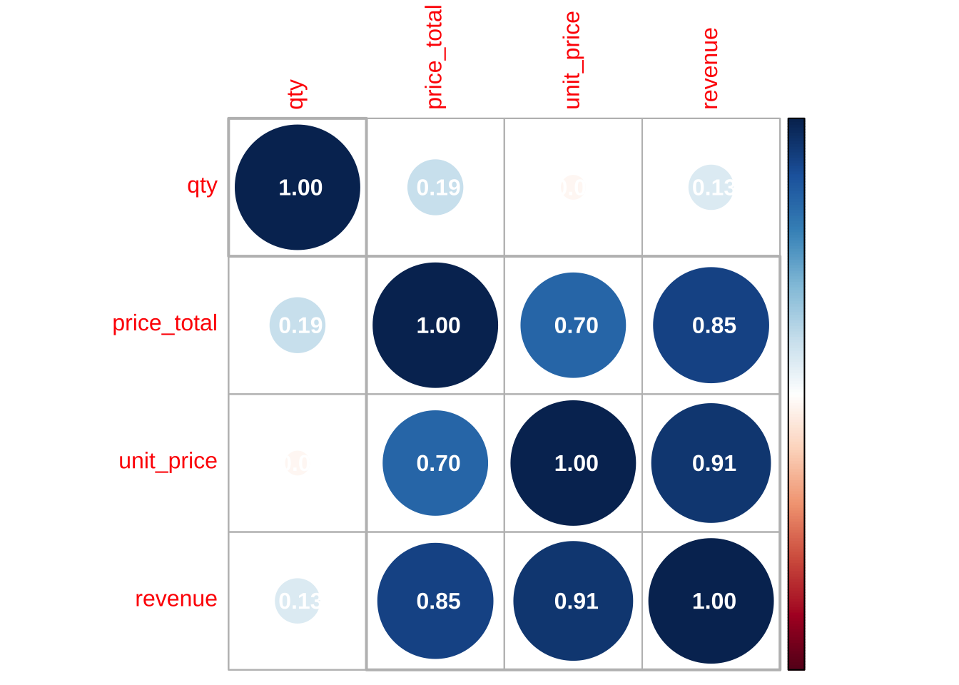

# Verteilung des Umsatzes prüfen
daten %>% 
  ggplot(mapping = aes(x = revenue)) +
  geom_histogram(bins = 50, fill = "#9FC131") +
  scale_x_log10() +
  labs(x = "Umsatz (log10)", 
       y = "Anzahl") +
  theme_dv()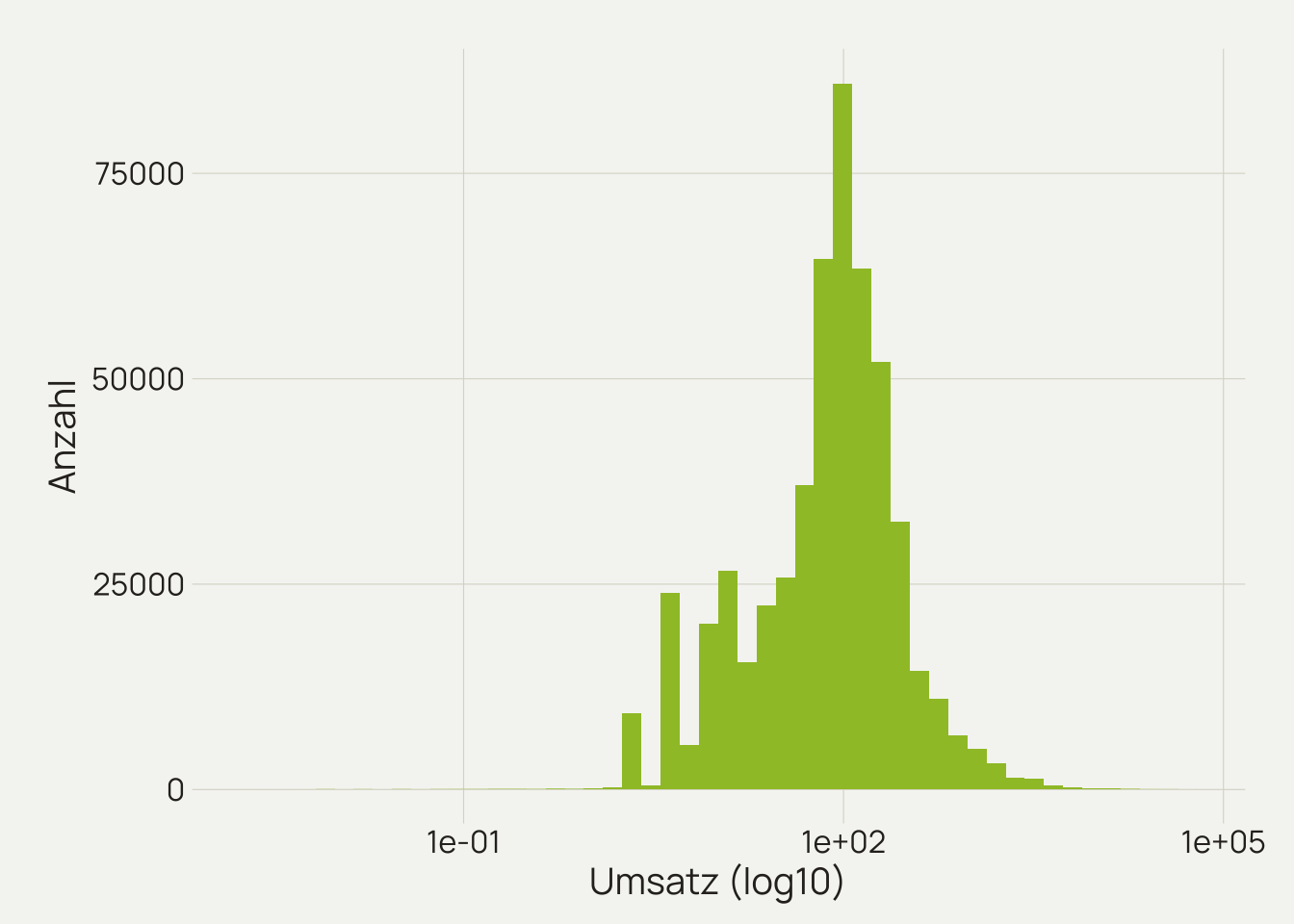

daten %>% 
  mutate(dept = as_factor(dept), 
         dept = fct_recode(dept, "dept_1" = "department_1", "dept_2" = "department_2", 
                           "dept_3" = "department_3", "dept_4" = "department_4", 
                           "dept_5" = "department_5", "dept_6" = "department_6", 
                           "dept_7" = "department_7", "dept_8" = "department_8", 
                           "dept_9" = "department_9")) %>% 
  ggplot(mapping = aes(x = as_factor(dept), y = revenue)) +
  geom_boxplot() +
  scale_y_log10() +
  labs(x = "Department", 
       y = "Umsatz (log10)") +
  theme_dv()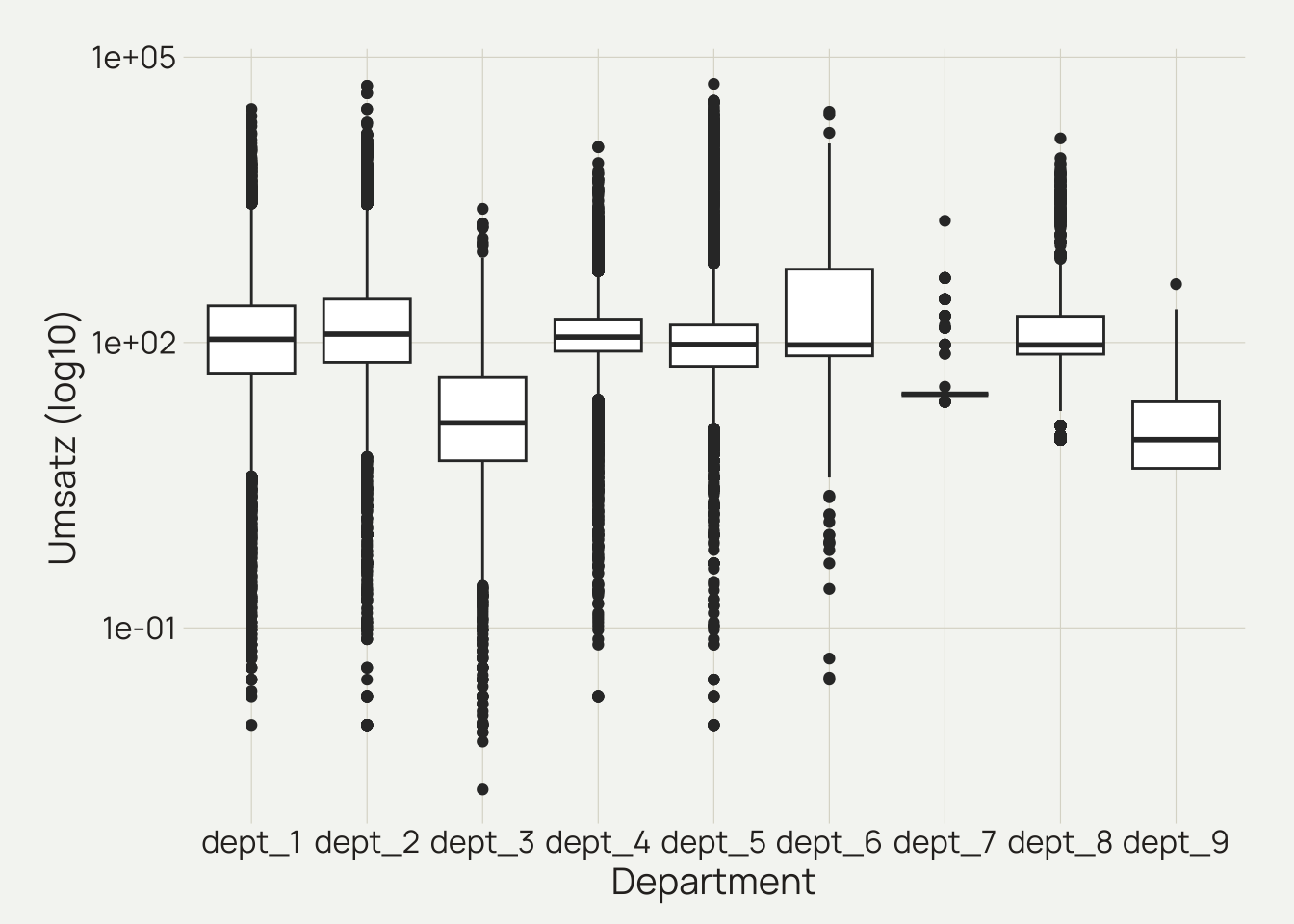

daten %>% 
  ggplot(mapping = aes(x = revenue, y = qty)) +
  geom_point() +
  labs(x = "Umsatz", 
       y = "QTY") +
  theme_dv()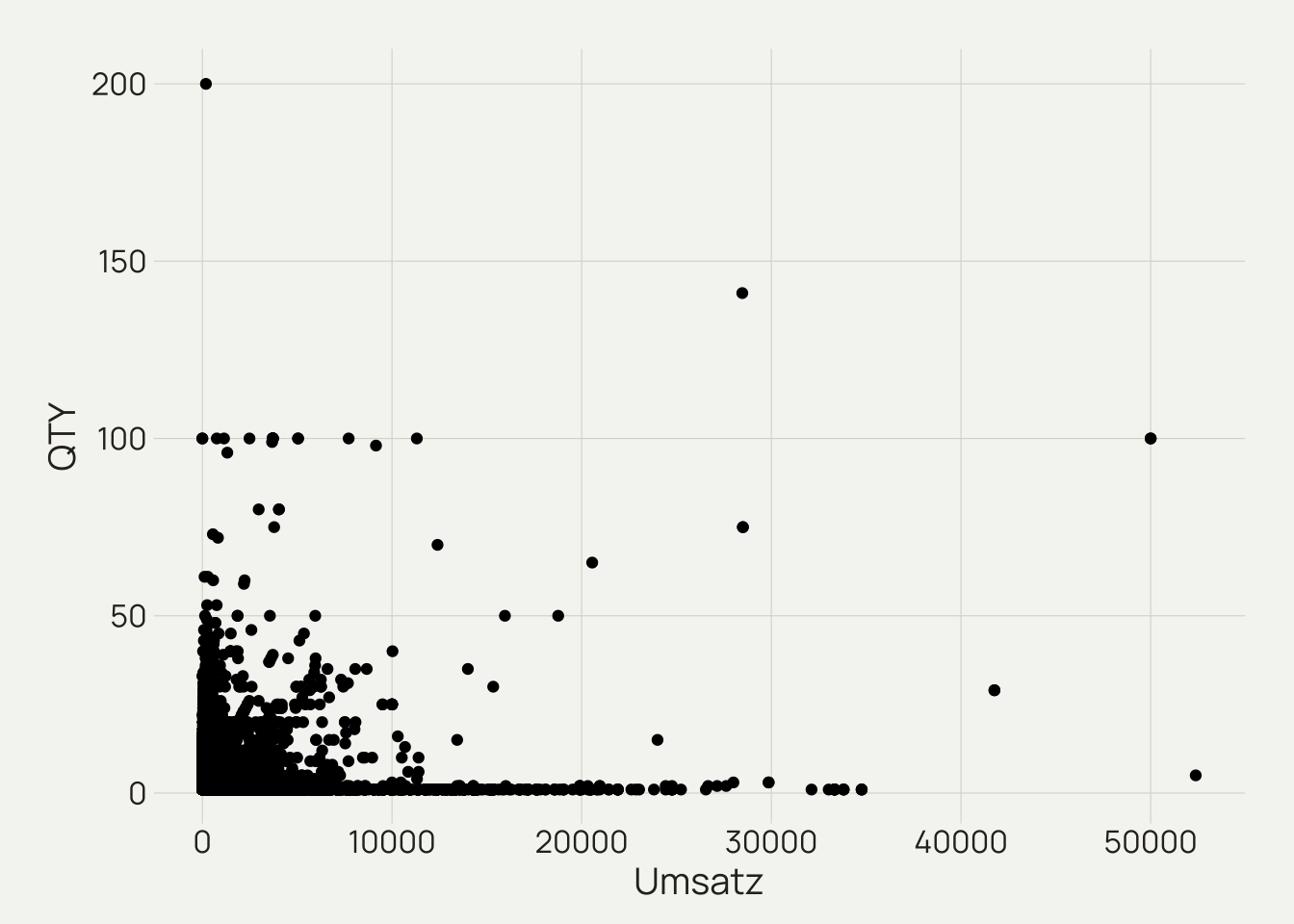

skim(daten)

Data summary

Name	daten
Number of rows	530765
Number of columns	14
_______________________
Column type frequency:
character	9
Date	1
numeric	4
________________________
Group variables	None

Variable type: character

skim_variable	n_missing	complete_rate	min	max	empty	n_unique	whitespace
store_name	0	1	7	7	0	8	0
dept	0	1	12	12	0	9	0
family	0	1	8	9	0	99	0
subfamily	0	1	11	13	0	443	0
section	0	1	9	10	0	55	0
brand	0	1	7	9	0	563	0
size	0	1	6	9	0	2082	0
color	0	1	7	10	0	2977	0
product	0	1	5	9	0	40016	0

Variable type: Date

skim_variable	n_missing	complete_rate	min	max	median	n_unique
date	0	1	2021-01-01	2023-07-30	2022-04-19	941

Variable type: numeric

skim_variable	n_missing	complete_rate	mean	sd	p0	p25	p50	p75	p100	hist
unit_price	0	1	179.77	575.12	0	30.00	90.00	169.00	36500.00	▇▁▁▁▁
revenue	0	1	170.82	566.93	0	33.71	85.71	160.95	52375.71	▇▁▁▁▁
price_total	0	1	196.18	852.26	0	39.00	95.00	180.00	249900.00	▇▁▁▁▁
qty	0	1	1.25	1.41	1	1.00	1.00	1.00	200.00	▇▁▁▁▁

Feature Engineering

Neue Prädiktorwerte erstellen

daten_grp <- 
  daten %>% 
  group_by(date, dept, family, subfamily, section, brand) %>% 
  summarise(total_rev = sum(revenue)) %>% 
  mutate(yearmonth = yearmonth(date))

`summarise()` has grouped output by 'date', 'dept', 'family', 'subfamily',
'section'. You can override using the `.groups` argument.

daten_grp <- 
  daten_grp %>% 
  group_by(yearmonth, dept, family, subfamily, section, brand) %>% 
  summarise(total_rev = sum(total_rev))

`summarise()` has grouped output by 'yearmonth', 'dept', 'family', 'subfamily',
'section'. You can override using the `.groups` argument.

daten_grp <- 
  daten_grp %>% 
  as_tsibble(key = c(dept, family, subfamily, section, brand), 
             index = yearmonth) %>% 
  fill_gaps(.full = TRUE)

daten_erw <- 
  daten_grp %>% 
  group_by(dept, family, subfamily, section, brand) %>% 
  mutate(trend = seq(1, n(), 1))

daten_erw$month <- 
  as.character(month(x = daten_erw$yearmonth, 
                     label = TRUE))

daten_erw <- 
  daten_erw %>% 
  arrange(yearmonth)

daten_erw_prognose <- 
  daten_erw %>% 
  group_by(dept, family, subfamily, section, brand) %>% 
  mutate(mean_rev = mean(total_rev), 
         sd_rev = sd(total_rev), 
         min_rev = min(total_rev), 
         max_rev = max(total_rev)) %>% 
  ungroup()

tail(daten_erw_prognose)

# A tsibble: 6 x 13 [1M]
# Key:       dept, family, subfamily, section, brand [6]
  yearmonth dept   family subfamily section brand total_rev trend month mean_rev
      <mth> <chr>  <chr>  <chr>     <chr>   <chr>     <dbl> <dbl> <chr>    <dbl>
1  2023 Jul depar… famil… subfamil… sectio… bran…        NA    31 Jul         NA
2  2023 Jul depar… famil… subfamil… sectio… bran…        NA    31 Jul         NA
3  2023 Jul depar… famil… subfamil… sectio… bran…        NA    31 Jul         NA
4  2023 Jul depar… famil… subfamil… sectio… bran…        NA    31 Jul         NA
5  2023 Jul depar… famil… subfamil… sectio… bran…        NA    31 Jul         NA
6  2023 Jul depar… famil… subfamil… sectio… bran…        NA    31 Jul         NA
# ℹ 3 more variables: sd_rev <dbl>, min_rev <dbl>, max_rev <dbl>

daten_erw_prognose <- 
  daten_erw_prognose %>% 
  mutate(across(.cols = where(is.numeric), 
                function(x) ifelse(test = is.na(x), 
                                   yes = 0, 
                                   no = x))) %>% 
  as_tibble()

tail(daten_erw_prognose)

# A tibble: 6 × 13
  yearmonth dept   family subfamily section brand total_rev trend month mean_rev
      <mth> <chr>  <chr>  <chr>     <chr>   <chr>     <dbl> <dbl> <chr>    <dbl>
1  2023 Jul depar… famil… subfamil… sectio… bran…         0    31 Jul          0
2  2023 Jul depar… famil… subfamil… sectio… bran…         0    31 Jul          0
3  2023 Jul depar… famil… subfamil… sectio… bran…         0    31 Jul          0
4  2023 Jul depar… famil… subfamil… sectio… bran…         0    31 Jul          0
5  2023 Jul depar… famil… subfamil… sectio… bran…         0    31 Jul          0
6  2023 Jul depar… famil… subfamil… sectio… bran…         0    31 Jul          0
# ℹ 3 more variables: sd_rev <dbl>, min_rev <dbl>, max_rev <dbl>

Daten aufteilen

# 80/20-Aufteilung der Daten
daten_teilen <- 
  initial_time_split(data = daten_erw_prognose, 
                     prop = 0.8)

train_daten <- training(x = daten_teilen)
test_daten <- testing(x = daten_teilen)

cat("Umfang Trainingsdaten:", 
    dim(train_daten), 
    "\nUmfang Testdaten:", 
    dim(test_daten))

Umfang Trainingsdaten: 61603 13 
Umfang Testdaten: 15401 13

recipes

train_daten_rp <- 
  train_daten %>% 
  select(dept:month, mean_rev:max_rev)

# Basis-Rezept
rezept <- 
  recipe(formula = total_rev ~ ., 
         data = train_daten_rp) %>% 
  # Zeichenprädiktoren in Faktoren umwandeln
  step_string2factor(all_nominal_predictors()) %>% 
  # Sicherstellen, dass Faktoren in Training und Testing konsistente Werte aufweisen
  step_novel(all_nominal_predictors()) %>% 
  # Fehlende Werte ergänzen
  # step_impute_median(all_numeric_predictors()) %>% # Alternative: step_impute_mean
  # step_impute_mode(all_nominal_predictors()) %>% 
  # Ausreisser bei numerischen Werten «entschärfen» & Varianz stabilisieren
  step_log() %>% 
  # Selten vorkommende Werte in Sammelstufe umwandeln
  step_other(dept, threshold = 0.07, id = "dept_id") %>% 
  step_other(family, threshold = 0.07, id = "family_id") %>% 
  step_other(subfamily, threshold = 0.07, id = "subfamily_id") %>% 
  step_other(section, threshold = 0.07, id = "section_id") %>% 
  step_other(brand, threshold = 0.07, id = "brand_id") %>% 
  # Fehlende Faktorstufen «unbekannt» zuweisen
  step_unknown(all_nominal_predictors()) %>% 
  # Dummy-Kodierung für Modelle, die numerische Eingaben benötigen, z.B. glmnet, xgboost, keras etc.
  step_dummy(all_nominal_predictors()) %>% 
  # Numerische Variablen mit Varianz Null entfernen; Alternative: step_nzv()
  step_zv(all_numeric_predictors()) %>% 
  # Normalisieren numerischer Prädiktoren (glmnet / neural nets)
  # step_normalize(all_numeric_predictors()) %>% 
  # Hoch korrelierte Variablen entfernen
  # step_corr(all_numeric_predictors(), threshold = 0.7) %>% 
  # Ausreisser bei numerischen Werten «entschärfen»
  step_poly(mean_rev:max_rev) %>% 
  step_YeoJohnson(all_numeric_predictors(), -contains("trend")) # %>% 
  # Datumsspalte neue Rolle zuweisen
  # update_role(date, new_role = "datum")

Modell erstellen und anpassen

Modell erstellen

model_lm <- 
  linear_reg() %>% 
  set_engine("lm")

model_tree <- 
  decision_tree(tree_depth = tune(), 
                min_n = tune()) %>% 
  set_engine("rpart") %>% 
  set_mode("regression")

# Ausgeführten Code am Beispiel von decision_tree()
model_tree %>% 
  translate()

Decision Tree Model Specification (regression)

Main Arguments:
  tree_depth = tune()
  min_n = tune()

Computational engine: rpart 

Model fit template:
rpart::rpart(formula = missing_arg(), data = missing_arg(), weights = missing_arg(), 
    maxdepth = tune(), minsplit = min_rows(tune(), data))

model_boost <- 
  boost_tree(
    mode = "regression", 
    engine = "xgboost", 
    mtry = tune(), 
    min_n = tune(), 
    tree_depth = tune(), 
    learn_rate = tune()
  )

model_glmnet <- 
  linear_reg(penalty = tune(), 
             mixture = tune()) %>% 
  set_engine("glmnet")

# Modellspezifikation am Beispiel von "glmnet"
model_glmnet

Linear Regression Model Specification (regression)

Main Arguments:
  penalty = tune()
  mixture = tune()

Computational engine: glmnet 

Leistungstest

fit_lm <- 
  model_lm %>% 
  fit(formula = total_rev ~ mean_rev + sd_rev + min_rev + max_rev, 
      data = train_daten)

fit_lm

parsnip model object


Call:
stats::lm(formula = total_rev ~ mean_rev + sd_rev + min_rev + 
    max_rev, data = data)

Coefficients:
(Intercept)     mean_rev       sd_rev      min_rev      max_rev  
   633.9410       0.7063      -0.2420      -0.1065       0.1731  

tidy(x = fit_lm)

# A tibble: 5 × 5
  term        estimate std.error statistic   p.value
  <chr>          <dbl>     <dbl>     <dbl>     <dbl>
1 (Intercept)  634.      17.9        35.3  6.90e-271
2 mean_rev       0.706    0.0425     16.6  7.23e- 62
3 sd_rev        -0.242    0.0523     -4.63 3.65e-  6
4 min_rev       -0.107    0.0850     -1.25 2.10e-  1
5 max_rev        0.173    0.0137     12.7  1.10e- 36

Workflow

Workflow (Pipeline) festlegen

wf_lm <- 
  workflow() %>% 
  add_recipe(recipe = rezept) %>% 
  add_model(spec = model_lm)

wf_tree <- 
  workflow() %>% 
  add_recipe(recipe = rezept) %>% 
  add_model(spec = model_tree)

wf_boost <- 
  workflow() %>% 
  add_recipe(recipe = rezept) %>% 
  add_model(spec = model_boost)

wf_glmnet <- 
  workflow() %>% 
  add_recipe(recipe = rezept) %>% 
  add_model(spec = model_glmnet)

Leistungstest

fit(object = wf_lm, 
    data = train_daten)

══ Workflow [trained] ══════════════════════════════════════════════════════════
Preprocessor: Recipe
Model: linear_reg()

── Preprocessor ────────────────────────────────────────────────────────────────
13 Recipe Steps

• step_string2factor()
• step_novel()
• step_log()
• step_other()
• step_other()
• step_other()
• step_other()
• step_other()
• step_unknown()
• step_dummy()
• ...
• and 3 more steps.

── Model ───────────────────────────────────────────────────────────────────────

Call:
stats::lm(formula = ..y ~ ., data = data)

Coefficients:
       (Intercept)               trend   dept_department_2   dept_department_3  
           -391.76               15.83              416.92             -272.28  
 dept_department_4   dept_department_5          dept_other     family_family_8  
            465.64              -26.48               98.64             -302.86  
      family_other     subfamily_other  section_section_11   section_section_4  
            300.05              543.82             -198.52             -613.50  
 section_section_5   section_section_7       section_other         brand_other  
            -64.33              109.39              -84.36              395.05  
         month_Aug           month_Dec           month_Feb           month_Jan  
           -123.42              857.47              268.07              509.82  
         month_Jul           month_Jun           month_Mar           month_May  
            -80.80             -367.01              199.37             -105.18  
         month_Nov           month_Oct           month_Sep     mean_rev_poly_1  
            577.13              429.96              -62.63           732818.50  
   mean_rev_poly_2       sd_rev_poly_1       sd_rev_poly_2      min_rev_poly_1  
        -331283.68            13710.50           -45090.63           -77961.82  
    min_rev_poly_2      max_rev_poly_1      max_rev_poly_2  
         -56585.82           491168.00           485749.33  

Beste Parameter finden

daten_angew <- 
  rezept %>% 
  prep() %>% 
  bake(new_data = NULL)

param_tree <- 
  hardhat::extract_parameter_set_dials(x = wf_tree) %>% 
  finalize(daten_angew)

param_boost <- 
  hardhat::extract_parameter_set_dials(x = wf_boost) %>% 
  finalize(daten_angew)

param_glmnet <- 
  hardhat::extract_parameter_set_dials(x = wf_glmnet) %>% 
  finalize(daten_angew)

Resampling

Time-based Resampling

train_daten$date <- 
  as.Date(x = train_daten$yearmonth)

train_resampling <- 
  sliding_period(data = train_daten, 
                 index = date, 
                 period = "month", 
                 lookback = Inf, 
                 assess_stop = 3, 
                 skip = 4, 
                 step = 3)

# Alternative:
# train_daten %>% 
  # group_by(yearmonth) %>% 
  # summarise(anzahl_zeilen = n())

# train_resampling <- 
  # sliding_window(data = train_daten, 
                 # lookback = (2484 * 3), 
                 # assess_stop = (2484 * 3), 
                 # step = (2484 * 3))

analysis(x = train_resampling$splits[[1]])

# A tibble: 12,420 × 14
   yearmonth dept  family subfamily section brand total_rev trend month mean_rev
       <mth> <chr> <chr>  <chr>     <chr>   <chr>     <dbl> <dbl> <chr>    <dbl>
 1  2021 Jan depa… famil… subfamil… sectio… bran…    17561.     1 Jan      6592.
 2  2021 Jan depa… famil… subfamil… sectio… bran…        0      1 Jan         0 
 3  2021 Jan depa… famil… subfamil… sectio… bran…        0      1 Jan         0 
 4  2021 Jan depa… famil… subfamil… sectio… bran…        0      1 Jan         0 
 5  2021 Jan depa… famil… subfamil… sectio… bran…    20056.     1 Jan      9597.
 6  2021 Jan depa… famil… subfamil… sectio… bran…        0      1 Jan         0 
 7  2021 Jan depa… famil… subfamil… sectio… bran…      450.     1 Jan         0 
 8  2021 Jan depa… famil… subfamil… sectio… bran…     3307.     1 Jan      4781.
 9  2021 Jan depa… famil… subfamil… sectio… bran…      502.     1 Jan         0 
10  2021 Jan depa… famil… subfamil… sectio… bran…     3733.     1 Jan         0 
# ℹ 12,410 more rows
# ℹ 4 more variables: sd_rev <dbl>, min_rev <dbl>, max_rev <dbl>, date <date>

assessment(x = train_resampling$splits[[1]])

# A tibble: 7,452 × 14
   yearmonth dept  family subfamily section brand total_rev trend month mean_rev
       <mth> <chr> <chr>  <chr>     <chr>   <chr>     <dbl> <dbl> <chr>    <dbl>
 1  2021 Jun depa… famil… subfamil… sectio… bran…     2036.     6 Jun      6592.
 2  2021 Jun depa… famil… subfamil… sectio… bran…        0      6 Jun         0 
 3  2021 Jun depa… famil… subfamil… sectio… bran…        0      6 Jun         0 
 4  2021 Jun depa… famil… subfamil… sectio… bran…        0      6 Jun         0 
 5  2021 Jun depa… famil… subfamil… sectio… bran…      849.     6 Jun      9597.
 6  2021 Jun depa… famil… subfamil… sectio… bran…        0      6 Jun         0 
 7  2021 Jun depa… famil… subfamil… sectio… bran…        0      6 Jun         0 
 8  2021 Jun depa… famil… subfamil… sectio… bran…     2083.     6 Jun      4781.
 9  2021 Jun depa… famil… subfamil… sectio… bran…        0      6 Jun         0 
10  2021 Jun depa… famil… subfamil… sectio… bran…        0      6 Jun         0 
# ℹ 7,442 more rows
# ℹ 4 more variables: sd_rev <dbl>, min_rev <dbl>, max_rev <dbl>, date <date>

Leistungstest

# fit_resamples am Beispiel von "lm" ohne angepasste Parameter
res_lm <- 
  fit_resamples(
    object = wf_lm, 
    resamples = train_resampling, 
    control = control_resamples(
      verbose = FALSE, 
      save_pred = TRUE, 
      save_workflow = TRUE))

res_lm

# Resampling results
# Sliding period resampling 
# A tibble: 6 × 5
  splits               id     .metrics         .notes           .predictions
  <list>               <chr>  <list>           <list>           <list>      
1 <split [12420/7452]> Slice1 <tibble [2 × 4]> <tibble [1 × 4]> <tibble>    
2 <split [19872/7452]> Slice2 <tibble [2 × 4]> <tibble [1 × 4]> <tibble>    
3 <split [27324/7452]> Slice3 <tibble [2 × 4]> <tibble [1 × 4]> <tibble>    
4 <split [34776/7452]> Slice4 <tibble [2 × 4]> <tibble [0 × 4]> <tibble>    
5 <split [42228/7452]> Slice5 <tibble [2 × 4]> <tibble [0 × 4]> <tibble>    
6 <split [49680/7452]> Slice6 <tibble [2 × 4]> <tibble [0 × 4]> <tibble>    

There were issues with some computations:

  - Warning(s) x3: prediction from rank-deficient fit; consider predict(., rankdefic...

Run `show_notes(.Last.tune.result)` for more information.

res_tree <- 
  tune_grid(
    object = wf_tree, 
    resamples = train_resampling, 
    param_info = param_tree, 
    grid = 10, 
    control = control_grid(
      verbose = FALSE, 
      save_pred = TRUE, 
      save_workflow = TRUE)
  )

res_boost <- 
  tune_grid(
    object = wf_boost, 
    resamples = train_resampling, 
    param_info = param_boost, 
    grid = 10, 
    control = control_grid(
      verbose = FALSE, 
      save_pred = TRUE, 
      save_workflow = TRUE)
  )

res_glmnet <- 
  tune_grid(
    object = wf_glmnet, 
    resamples = train_resampling, 
    param_info = param_glmnet, 
    grid = 10, 
    control = control_grid(
      verbose = FALSE, 
      save_pred = TRUE, 
      save_workflow = TRUE)
  )

Visuelle Diagnose mit autoplot()

autoplot(object = res_tree, 
         type = "marginals", 
         metric = "rmse")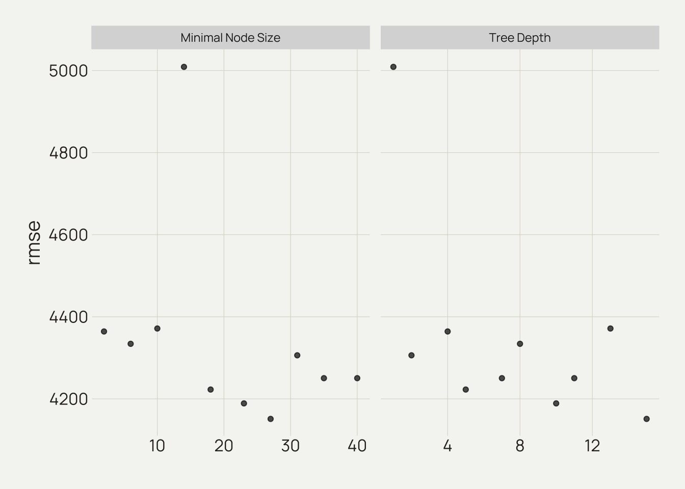

Vorhersagen vergleichen

# Vorhersagen für "lm"
collect_predictions(x = res_lm)

# A tibble: 44,712 × 5
   .pred id     total_rev  .row .config        
   <dbl> <chr>      <dbl> <int> <chr>          
 1 4896. Slice1     2036. 12421 pre0_mod0_post0
 2  260. Slice1        0  12422 pre0_mod0_post0
 3  260. Slice1        0  12423 pre0_mod0_post0
 4  260. Slice1        0  12424 pre0_mod0_post0
 5 6275. Slice1      849. 12425 pre0_mod0_post0
 6  260. Slice1        0  12426 pre0_mod0_post0
 7  260. Slice1        0  12427 pre0_mod0_post0
 8 3930. Slice1     2083. 12428 pre0_mod0_post0
 9  260. Slice1        0  12429 pre0_mod0_post0
10  260. Slice1        0  12430 pre0_mod0_post0
# ℹ 44,702 more rows

# Vorhersagen für decision_tree()
collect_predictions(x = res_tree)

# A tibble: 447,120 × 7
   .pred id     total_rev  .row tree_depth min_n .config         
   <dbl> <chr>      <dbl> <int>      <int> <int> <chr>           
 1  774. Slice1     2036. 12421          1    14 pre0_mod01_post0
 2  774. Slice1        0  12422          1    14 pre0_mod01_post0
 3  774. Slice1        0  12423          1    14 pre0_mod01_post0
 4  774. Slice1        0  12424          1    14 pre0_mod01_post0
 5  774. Slice1      849. 12425          1    14 pre0_mod01_post0
 6  774. Slice1        0  12426          1    14 pre0_mod01_post0
 7  774. Slice1        0  12427          1    14 pre0_mod01_post0
 8  774. Slice1     2083. 12428          1    14 pre0_mod01_post0
 9  774. Slice1        0  12429          1    14 pre0_mod01_post0
10  774. Slice1        0  12430          1    14 pre0_mod01_post0
# ℹ 447,110 more rows

# Vorhersagen für boost_tree()
collect_predictions(x = res_boost)

# A tibble: 447,120 × 9
    .pred id     total_rev  .row  mtry min_n tree_depth learn_rate .config      
    <dbl> <chr>      <dbl> <int> <int> <int>      <int>      <dbl> <chr>        
 1  6443. Slice1     2036. 12421     1    23          5      0.167 pre0_mod01_p…
 2   436. Slice1        0  12422     1    23          5      0.167 pre0_mod01_p…
 3   436. Slice1        0  12423     1    23          5      0.167 pre0_mod01_p…
 4   436. Slice1        0  12424     1    23          5      0.167 pre0_mod01_p…
 5 13691. Slice1      849. 12425     1    23          5      0.167 pre0_mod01_p…
 6   436. Slice1        0  12426     1    23          5      0.167 pre0_mod01_p…
 7   436. Slice1        0  12427     1    23          5      0.167 pre0_mod01_p…
 8  3617. Slice1     2083. 12428     1    23          5      0.167 pre0_mod01_p…
 9   436. Slice1        0  12429     1    23          5      0.167 pre0_mod01_p…
10   436. Slice1        0  12430     1    23          5      0.167 pre0_mod01_p…
# ℹ 447,110 more rows

# Vorhersagen für "glmnet"
collect_predictions(x = res_glmnet)

# A tibble: 447,120 × 7
   .pred id     total_rev  .row      penalty mixture .config         
   <dbl> <chr>      <dbl> <int>        <dbl>   <dbl> <chr>           
 1 4890. Slice1     2036. 12421 0.0000000001   0.367 pre0_mod01_post0
 2  232. Slice1        0  12422 0.0000000001   0.367 pre0_mod01_post0
 3  232. Slice1        0  12423 0.0000000001   0.367 pre0_mod01_post0
 4  232. Slice1        0  12424 0.0000000001   0.367 pre0_mod01_post0
 5 6021. Slice1      849. 12425 0.0000000001   0.367 pre0_mod01_post0
 6  232. Slice1        0  12426 0.0000000001   0.367 pre0_mod01_post0
 7  232. Slice1        0  12427 0.0000000001   0.367 pre0_mod01_post0
 8 3865. Slice1     2083. 12428 0.0000000001   0.367 pre0_mod01_post0
 9  232. Slice1        0  12429 0.0000000001   0.367 pre0_mod01_post0
10  232. Slice1        0  12430 0.0000000001   0.367 pre0_mod01_post0
# ℹ 447,110 more rows

Metriken

# Leistungskennzahlen für "lm"
collect_metrics(x = res_lm)

# A tibble: 2 × 6
  .metric .estimator     mean     n  std_err .config        
  <chr>   <chr>         <dbl> <int>    <dbl> <chr>          
1 rmse    standard   4068.        6 388.     pre0_mod0_post0
2 rsq     standard      0.557     6   0.0485 pre0_mod0_post0

# Leistungskennzahlen für decision_tree()
collect_metrics(x = res_tree)

# A tibble: 20 × 8
   tree_depth min_n .metric .estimator     mean     n  std_err .config         
        <int> <int> <chr>   <chr>         <dbl> <int>    <dbl> <chr>           
 1          1    14 rmse    standard   5009.        6 458.     pre0_mod01_post0
 2          1    14 rsq     standard      0.299     6   0.0542 pre0_mod01_post0
 3          2    31 rmse    standard   4306.        6 380.     pre0_mod02_post0
 4          2    31 rsq     standard      0.475     6   0.0471 pre0_mod02_post0
 5          4     2 rmse    standard   4364.        6 430.     pre0_mod03_post0
 6          4     2 rsq     standard      0.500     6   0.0342 pre0_mod03_post0
 7          5    18 rmse    standard   4223.        6 374.     pre0_mod04_post0
 8          5    18 rsq     standard      0.523     6   0.0471 pre0_mod04_post0
 9          7    35 rmse    standard   4250.        6 307.     pre0_mod05_post0
10          7    35 rsq     standard      0.506     6   0.0406 pre0_mod05_post0
11          8     6 rmse    standard   4334.        6 423.     pre0_mod06_post0
12          8     6 rsq     standard      0.504     6   0.0399 pre0_mod06_post0
13         10    23 rmse    standard   4189.        6 362.     pre0_mod07_post0
14         10    23 rsq     standard      0.526     6   0.0480 pre0_mod07_post0
15         11    40 rmse    standard   4250.        6 307.     pre0_mod08_post0
16         11    40 rsq     standard      0.506     6   0.0406 pre0_mod08_post0
17         13    10 rmse    standard   4371.        6 424.     pre0_mod09_post0
18         13    10 rsq     standard      0.498     6   0.0434 pre0_mod09_post0
19         15    27 rmse    standard   4151.        6 340.     pre0_mod10_post0
20         15    27 rsq     standard      0.535     6   0.0427 pre0_mod10_post0

# Leistungskennzahlen für boost_tree()
collect_metrics(x = res_boost)

# A tibble: 20 × 10
    mtry min_n tree_depth learn_rate .metric .estimator     mean     n  std_err
   <int> <int>      <int>      <dbl> <chr>   <chr>         <dbl> <int>    <dbl>
 1     1    23          5    0.167   rmse    standard   4399.        6 508.    
 2     1    23          5    0.167   rsq     standard      0.509     6   0.0198
 3     4     2         10    0.0129  rmse    standard   5280.        6 621.    
 4     4     2         10    0.0129  rsq     standard      0.565     6   0.0468
 5     8    27         13    0.00190 rmse    standard   5761.        6 624.    
 6     8    27         13    0.00190 rsq     standard      0.520     6   0.0301
 7    12    35          2    0.00359 rmse    standard   5717.        6 623.    
 8    12    35          2    0.00359 rsq     standard      0.481     6   0.0290
 9    16    40         11    0.0880  rmse    standard   4280.        6 482.    
10    16    40         11    0.0880  rsq     standard      0.511     6   0.0293
11    19     6          1    0.00681 rmse    standard   5648.        6 622.    
12    19     6          1    0.00681 rsq     standard      0.316     6   0.0547
13    23    10          7    0.316   rmse    standard   3999.        6 393.    
14    23    10          7    0.316   rsq     standard      0.568     6   0.0431
15    27    14         15    0.0245  rmse    standard   4887.        6 595.    
16    27    14         15    0.0245  rsq     standard      0.538     6   0.0372
17    31    18          8    0.001   rmse    standard   5790.        6 623.    
18    31    18          8    0.001   rsq     standard      0.502     6   0.0419
19    35    31          4    0.0464  rmse    standard   4581.        6 560.    
20    35    31          4    0.0464  rsq     standard      0.504     6   0.0214
# ℹ 1 more variable: .config <chr>

# Leistungskennzahlen für "glmnet"
collect_metrics(x = res_glmnet)

# A tibble: 20 × 8
         penalty mixture .metric .estimator     mean     n  std_err .config     
           <dbl>   <dbl> <chr>   <chr>         <dbl> <int>    <dbl> <chr>       
 1 0.0000000001    0.367 rmse    standard   4040.        6 375.     pre0_mod01_…
 2 0.0000000001    0.367 rsq     standard      0.560     6   0.0477 pre0_mod01_…
 3 0.00000000129   0.789 rmse    standard   4038.        6 376.     pre0_mod02_…
 4 0.00000000129   0.789 rsq     standard      0.560     6   0.0480 pre0_mod02_…
 5 0.0000000167    0.05  rmse    standard   4028.        6 374.     pre0_mod03_…
 6 0.0000000167    0.05  rsq     standard      0.561     6   0.0474 pre0_mod03_…
 7 0.000000215     0.472 rmse    standard   4040.        6 375.     pre0_mod04_…
 8 0.000000215     0.472 rsq     standard      0.560     6   0.0478 pre0_mod04_…
 9 0.00000278      0.894 rmse    standard   4036.        6 376.     pre0_mod05_…
10 0.00000278      0.894 rsq     standard      0.561     6   0.0478 pre0_mod05_…
11 0.0000359       0.156 rmse    standard   4038.        6 376.     pre0_mod06_…
12 0.0000359       0.156 rsq     standard      0.560     6   0.0478 pre0_mod06_…
13 0.000464        0.578 rmse    standard   4036.        6 375.     pre0_mod07_…
14 0.000464        0.578 rsq     standard      0.561     6   0.0479 pre0_mod07_…
15 0.00599         1     rmse    standard   4037.        6 376.     pre0_mod08_…
16 0.00599         1     rsq     standard      0.561     6   0.0478 pre0_mod08_…
17 0.0774          0.261 rmse    standard   4041.        6 376.     pre0_mod09_…
18 0.0774          0.261 rsq     standard      0.559     6   0.0479 pre0_mod09_…
19 1               0.683 rmse    standard   4035.        6 374.     pre0_mod10_…
20 1               0.683 rsq     standard      0.561     6   0.0477 pre0_mod10_…

vier_modelle <- 
  as_workflow_set(lm = res_lm, 
                  glmnet = res_glmnet, 
                  tree = res_tree, 
                  boost = res_boost)

autoplot(object = vier_modelle, 
         rank_metric = "rmse", # Reihenfolge der Modelle
         metric = "rmse", # Metrik zum Visualisieren; Alternative: rsq
         select_best = TRUE) + # ein Punkt pro Workflow
  geom_text(mapping = aes(y = (mean - 800), label = wflow_id), 
            angle = 90, 
            hjust = 1) +
  ylim(2800, 5000) +
  theme(legend.position = "none")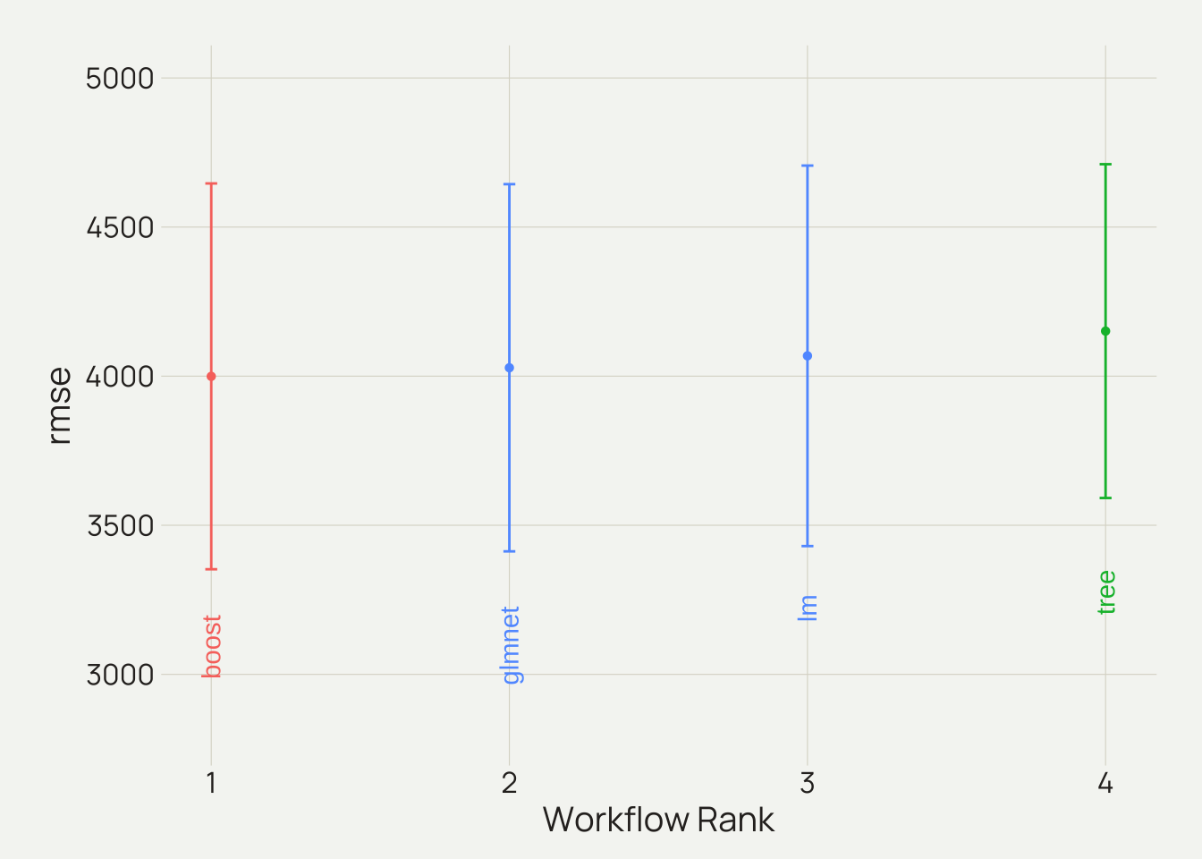

Workflow finalisieren

Bestes Modell auswählen

best_tree <- 
  select_best(x = res_tree, 
              metric = "rmse")

best_boost <- 
  select_best(x = res_boost, 
              metric = "rmse")

best_glmnet <- 
  select_best(x = res_glmnet, 
              metric = "rmse")

Bestes Modell anwenden

final_fit_lm <- 
  fit(object = wf_lm, 
      data = train_daten)

wf_final_tree <- 
  finalize_workflow(x = wf_tree, 
                    parameters = best_tree)
final_fit_tree <- 
  fit(object = wf_final_tree, 
      data = train_daten)

wf_final_boost <- 
  finalize_workflow(x = wf_boost, 
                    parameters = best_boost)
final_fit_boost <- 
  fit(object = wf_final_boost, 
      data = train_daten)

wf_final_glmnet <- 
  finalize_workflow(x = wf_glmnet, 
                    parameters = best_glmnet)
final_fit_glmnet <- 
  fit(object = wf_final_glmnet, 
      data = train_daten)

wf_final_glmnet

══ Workflow ════════════════════════════════════════════════════════════════════
Preprocessor: Recipe
Model: linear_reg()

── Preprocessor ────────────────────────────────────────────────────────────────
13 Recipe Steps

• step_string2factor()
• step_novel()
• step_log()
• step_other()
• step_other()
• step_other()
• step_other()
• step_other()
• step_unknown()
• step_dummy()
• ...
• and 3 more steps.

── Model ───────────────────────────────────────────────────────────────────────
Linear Regression Model Specification (regression)

Main Arguments:
  penalty = 1.66810053720006e-08
  mixture = 0.05

Computational engine: glmnet 

Vorhersagen mit endgültigen Modellen

pred_lm <- 
  test_daten %>% 
  bind_cols(., predict(object = final_fit_lm, 
                       new_data = .)) %>% 
  select(yearmonth, total_rev, .pred)

pred_tree <- 
  test_daten %>% 
  bind_cols(., predict(object = final_fit_tree, 
                       new_data = .)) %>% 
  select(yearmonth, total_rev, .pred)

pred_boost <- 
  test_daten %>% 
  bind_cols(., predict(object = final_fit_boost, 
                       new_data = .)) %>% 
  select(yearmonth, total_rev, .pred)

pred_glmnet <- 
  test_daten %>% 
  bind_cols(., predict(object = final_fit_glmnet, 
                       new_data = .)) %>% 
  select(yearmonth, total_rev, .pred)

Vorhersagequalität der Modelle

data.frame(model = c("lm", "tree", "boost", "glmnet"), 
           rmse = c(rmse(data = pred_lm, total_rev, .pred)$.estimate, 
                    rmse(data = pred_tree, total_rev, .pred)$.estimate, 
                    rmse(data = pred_boost, total_rev, .pred)$.estimate, 
                    rmse(data = pred_glmnet, total_rev, .pred)$.estimate))

   model     rmse
1     lm 6073.086
2   tree 6219.038
3  boost 6663.720
4 glmnet 6065.689